Simple Logistic Regression[Case Study]

Logic behind Simple Logistic Regression

Introduction :

The goal of the blogpost is to get the beginners started with fundamental concepts  of the Simple logistic regression concepts and quickly help them to build their first Simple logistic regression model.  We will mainly focus on learning to build your first logistic regression model . The data cleaning and preprocessing parts would be covered in detail in an upcoming post.

Logistic regression are one of the most fundamental and widely used Machine Learning Algorithm. Logistic regression is usually among the first few topics which people pick while learning predictive modeling. Don’t get confused with suffix “regression” in the algorithm name.  Logistic regression is not a regression algorithm but actually a probabilistic classification model.

Classification Machine Learning is a technique of learning where a particular instance is mapped against one of the many labels. The labels are prespecified to train your model . The machine learns the pattern from the data in such a way that the learned representation successfully  maps the original dimension to the suggested label/class without any more intervention from a human expert.

A logistic regression in its plain form is used to model relationship between one or more predictor variables to a binary categorical target variable. The target variable is marked as “1” and “0”. Since the target is binary hence we can call vanilla logistic regression as binary logistic regression. The binary logistic regression model is used to estimate the probability of a binary response based on one or more predictor (or independent) variables (features). For example, we may find that plants with a high level of a fungal infection (X1) fall into the category “the plant lives” (Y) less often than those plants with low level of infection. Thus, as the level of infection rises, the probability of plant living decreases.

Logistic regression is a linear model which can be subjected to nonlinear transforms.The logistic regression formula is derived from the standard linear equation for a straight line. The linear representation(-inf,+inf) is converted to a probability representation (0-1) using the sigmoidal curve.

How ever the purpose of using logistic regression in place of linear regression is that we want our classification score to be a number which can be easily interpreted in terms of probability whose entire range must sum to 1. Hence we need to represent the particular linear function in terms of another function which can squeeze the generated score between a continuous number between 0 and 1. Sigmoid is one function which does this. It squeezes any number generated by a function in this case a (w*x + b ) between 0 and 1.

Following is the graph for the sigmoidal function :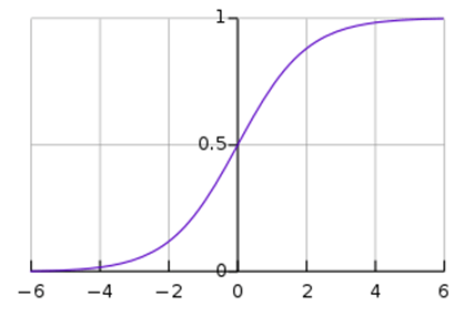

The equation for sigmoid function is :

S(x) = 1 / (1+e^-x)

It ensures that the generated number is always between 0 and 1 since the numerator is always smaller than the denominator by 1. See below,

S(x) = 1 / (1+e^-x) = e^x / (1+e^x)

Derivation from linear function to a sigmoid function :

The outcome in binomial logistic regression can be a 0 or a 1. The idea is then to estimate the probability of an outcome being a 1 or a 0. Given that the probability of the outcome being a 1 is given by p then the probability of it not occurring is given by 1-p.This can be seen as a special case of Binomial distribution called the Bernoulli distribution.

The idea in logistic regression is to cast the problem in form of generalized linear regression model.
ŷ = β₀ + β₁ x₁ + β_nx_n
where ŷ =predicted value, x= independent variables and the β are coefficients to be learnt.

This can be compactly expressed in vector form:
ŷ = β₀ + β₁ x₁ + β_nx_n
Then
ŷ = w_Tx

Logistic regression comes from the fact that linear regression can also be used to perform classification problem. Logistic Regression is part of a larger class of algorithms known as Generalized Linear Model (glm).This model was proposed as a means of using linear regression to the problems which were not directly suited for application of linear regression.

The fundamental equation of generalized linear model is:

g(E(y)) = α + βx1 + γx2

here g() is a link function.The role of link function is to ‘link’ the expectation of y to linear predictor.

GLM does not assume a linear relationship between dependent and independent variables. However, it assumes a linear relationship between link function and independent variables .

Hence, logistic regression as a special case of linear regression and when the outcome variable is categorical, where we are using log of odds as dependent variable.

In simple words, it predicts the probability of occurrence of an event by fitting data to a logit function. Thus the logit function acts like a link between logistic regression and linear regression.

odds(p) = p/1-p

logit(p) = log(p/1-p)

logit(p) = ŷ = w_Tx

Taking the natural exponential on both sides gives:

logit(p) = log(p/1-p)

e_logit(p) = p/1-p

Add 1 on both sides

e_ŷ +1= (p/1-p) + 1

e_ŷ +1= (1/1-p)

1-p = 1/e_ŷ+1

p = 1 – (1/e_ŷ +1)

p = e_ŷ/(e_ŷ+1)

p = 1/(1+e_-ŷ)

This looks like the sigmoid function isn’t it.

Enough of theory now let’s dive into the implementation  logistic regression .

We will use implementation provided by the python machine learning framework known as scikit-learn.

Problem Statement :

To build a simple logistic regression model for prediction of demand of bikes given the values about the wind speed.

Data details

==========================================
Bike Sharing Dataset
==========================================
The dataset is available at  “https://archive.ics.uci.edu/ml/datasets/bike+sharing+dataset”

=========================================
Background
=========================================

Bike sharing systems are new generation of traditional bike rentals where whole process from membership, rental and return
back has become automatic. Through these systems, user is able to easily rent a bike from a particular position and return
back at another position. Currently, there are about over 500 bike-sharing programs around the world which is composed of
over 500 thousands bicycles. Today, there exists great interest in these systems due to their important role in traffic,
environmental and health issues.

Apart from interesting real world applications of bike sharing systems, the characteristics of data being generated by
these systems make them attractive for the research. Opposed to other transport services such as bus or subway, the duration
of travel, departure and arrival position is explicitly recorded in these systems. This feature turns bike sharing system into
a virtual sensor network that can be used for sensing mobility in the city. Hence, it is expected that most of important
events in the city could be detected via monitoring these data.

=========================================
Data Set
=========================================
Bike-sharing rental process is highly correlated to the environmental and seasonal settings. For instance, weather conditions,
precipitation, day of week, season, hour of the day, etc. can affect the rental behaviors. The core data set is related to
the two-year historical log corresponding to years 2011 and 2012 from Capital Bikeshare system, Washington D.C., USA which is
publicly available in http://capitalbikeshare.com/system-data. We aggregated the data on two hourly and daily basis and then
extracted and added the corresponding weather and seasonal information. Weather information are extracted from http://www.freemeteo.com.

=========================================
Files
=========================================

– Readme.txt
– hour.csv : bike sharing counts aggregated on hourly basis. Records: 17379 hours
– day.csv – bike sharing counts aggregated on daily basis. Records: 731 days

=========================================
Dataset characteristics
=========================================
Both hour.csv and day.csv have the following fields, except hr which is not available in day.csv

– instant: record index
– dteday : date
– season : season (1:springer, 2:summer, 3:fall, 4:winter)
– yr : year (0: 2011, 1:2012)
– mnth : month ( 1 to 12)
– hr : hour (0 to 23)
– holiday : weather day is holiday or not (extracted from http://dchr.dc.gov/page/holiday-schedule)
– weekday : day of the week
– workingday : if day is neither weekend nor holiday is 1, otherwise is 0.
+ weathersit :
– 1: Clear, Few clouds, Partly cloudy, Partly cloudy
– 2: Mist + Cloudy, Mist + Broken clouds, Mist + Few clouds, Mist
– 3: Light Snow, Light Rain + Thunderstorm + Scattered clouds, Light Rain + Scattered clouds
– 4: Heavy Rain + Ice Pallets + Thunderstorm + Mist, Snow + Fog
– temp : Normalized temperature in Celsius. The values are divided to 41 (max)
– atemp: Normalized feeling temperature in Celsius. The values are divided to 50 (max)
– hum: Normalized humidity. The values are divided to 100 (max)
– windspeed: Normalized wind speed. The values are divided to 67 (max)
– casual: count of casual users
– registered: count of registered users
– cnt: count of total rental bikes including both casual and registered

=========================================
License
=========================================
Use of this dataset in publications must be cited to the following publication:

[1] Fanaee-T, Hadi, and Gama, Joao, “Event labeling combining ensemble detectors and background knowledge”, Progress in Artificial Intelligence (2013): pp. 1-15, Springer Berlin Heidelberg, doi:10.1007/s13748-013-0040-3.

@article{
year={2013},
issn={2192-6352},
journal={Progress in Artificial Intelligence},
doi={10.1007/s13748-013-0040-3},
title={Event labeling combining ensemble detectors and background knowledge},
url={http://dx.doi.org/10.1007/s13748-013-0040-3},
publisher={Springer Berlin Heidelberg},
keywords={Event labeling; Event detection; Ensemble learning; Background knowledge},
author={Fanaee-T, Hadi and Gama, Joao},
pages={1-15}
}

Python Implementation with code :

1. Import necessary libraries

Import the necessary modules from specific libraries.

import pandas as pd
from glob import glob
from sklearn.linear_model import LogisticRegression
from sklearn.cross_validation import train_test_split
from sklearn import metrics, cross_validation
from sklearn.metrics import  mean_squared_error, r2_score

1. Load the data set

Use pandas module to read the bike data from the file system. Check few records of the dataset.

data_list = glob('data/bike-sharing/*')
day_df = pd.read_csv(data_list[2])
day_df.head()

instant    dteday    season   yr             mnth       holiday   weekday workingday            weathersit               temp        atemp                hum         windspeed             casual     registered               cnt

0              1              2011-01-01             1              0              1              0              6              0              2              0.344167                0.363625 0.805833 0.160446 331          654          985

1              2              2011-01-02             1              0              1              0              0              0              2              0.363478                0.353739 0.696087 0.248539 131          670          801

2              3              2011-01-03             1              0              1              0              1              1              1              0.196364                0.189405 0.437273 0.248309 120          1229        1349

3              4              2011-01-04             1              0              1              0              2              1              1              0.200000                0.212122 0.590435 0.160296 108          1454        1562

4              5              2011-01-05             1              0              1              0              3              1              1              0.226957                0.229270 0.436957 0.186900 82            1518        1600

2. Identify the target variable and convert it into categorical variable

The problem we are solving is to model the demand of the bikes. If we observer in the dataset, the last column which says “cnt” gives us the total bikes used in particular day. This will be our target column. However this column contains continuous values. In order to build a logistic regression model we should have a target variable which is discrete. Hence let’s convert the particular column into a categorical column by thresholding it on a particular value. Let’s check five-num summary of the target column.

day_df.iloc[:,-1].describe()

count     731.000000
mean     4504.348837
std      1937.211452
min        22.000000
25%      3152.000000
50%      4548.000000
75%      5956.000000
max      8714.000000
Name: cnt, dtype: float64

This show that avg demand of the bike per day has been around 4504. Since we are trying to predict a number which shows a higher demand. Let’s pick a number close to the 50th percentile of the distribution. We fix a threshold of 4600  i.e. any number >4600 can be considered as high demand.

day_df['High'] = day_df.cnt.map(lambda x: 1 if x>4600 else 0)

2. Select the predictor feature and select the target variable

X =  day_df[['windspeed']]

y =  day_df['High']

3. Train test split :

X_train, X_test, y_train, y_test = train_test_split(X, y, test_size=0.3, random_state=12)

4. Training / model fitting

model = LogisticRegression()

model.fit(X_train, y_train)

5. Model parameters study :

predicted = model.predict(X_test)

# generate evaluation metrics

print(metrics.accuracy_score(y_test, predicted))

0.5727272727272728

The accuracy is ~58 % which is not a very good model. This is however expected in case of univariate logistic regression. Reason being one predictor variable might not be sufficient enough for making a decision. Model tuning , feature engineering , data preprocessing are few tricks which can help make our model better. The scope of the blog is however to learn how to create a model given a dataset. The model improvement will be covered in the next blogpost.

Predicting the Probability the count of bike demand to be high

Just for fun, let’s predict the probability of the bike demand for a random day not present in the dataset. The wind speed at that particular day is minimum and maximum. Expectation is when the wind speed is high people would prefer to ride less and  when the wind speed is low people would prefer to ride more .

Let’s validate the same with model.

Case 1 : when the wind speed is minimum

test_data = day_df.windspeed.min()

print(model.predict(test_data))

print(model.predict_proba(test_data))

[1]
[[0.44937194 0.55062806]]

This means that bike demand is on higher side and the confidence is ~55%.

Case 2 : when the wind speed is maximum

test_data = day_df.windspeed.max()

print(model.predict(test_data))

print(model.predict_proba(test_data))

[0]
[[0.64939015 0.35060985]]

This means that bike demand is on lower side and the confidence is ~65%.

Logistic Regression Assumptions :

* Binary logistic regression requires the dependent variable to be binary.

* For a binary regression, the factor level 1 of the dependent variable should represent the desired outcome.

* Meaningful variables should be included.

* The independent variables should be independent of each other.

* The feature are linearly related to the logits of the target variable.

* Sample size should be sufficient – at least 50 records per predictor