
Introduction :
The goal of the blogpost is to equip beginners with the basics of Decision Tree Regressor algorithm and quickly help them to build their first model. We will mainly focus on the modelling side of it. The data cleaning and preprocessing parts would be covered in detail in an upcoming post.

Source : https://chrisalbon.com/
In statistics, the mean squared error (MSE) or mean squared deviation (MSD) of an estimator (of a procedure for estimating an unobserved quantity) measures the average of the squares of the errors—that is, the average squared difference between the estimated values and what is estimated.
The MSE is a measure of the quality of an estimator—it is always non-negative, and values closer to zero are better.
The Mean Squared Error is given by:
Enough of theory , let’s start with implementation.
Problem Statement :
To predict the median prices of homes located in boston area given other attributes of the house.
Data details
Boston House Prices dataset
===========================
Notes:
Data Set Characteristics:
:Number of Instances: 506
:Number of Attributes: 13 numeric/categorical predictive
:Median Value (attribute 14) is usually the target
:Attribute Information (in order):
– CRIM per capita crime rate by town
– ZN proportion of residential land zoned for lots over 25,000 sq.ft.
– INDUS proportion of non-retail business acres per town
– CHAS Charles River dummy variable (= 1 if tract bounds river; 0 otherwise)
– NOX nitric oxides concentration (parts per 10 million)
– RM average number of rooms per dwelling
– AGE proportion of owner-occupied units built prior to 1940
– DIS weighted distances to five Boston employment centres
– RAD index of accessibility to radial highways
– TAX full-value property-tax rate per $10,000
– PTRATIO pupil-teacher ratio by town
– B 1000(Bk – 0.63)^2 where Bk is the proportion of blacks by town
– LSTAT % lower status of the population
– MEDV Median value of owner-occupied homes in $1000’s
:Missing Attribute Values: None
:Creator: Harrison, D. and Rubinfeld, D.L.
This is a copy of UCI ML housing dataset.
http://archive.ics.uci.edu/ml/datasets/Housing
This dataset was taken from the StatLib library which is maintained at Carnegie Mellon University.
The Boston house-price data of Harrison, D. and Rubinfeld, D.L. ‘Hedonic prices and the demand for clean air’, J. Environ. Economics & Management, vol.5, 81-102, 1978. Used in Belsley, Kuh & Welsch, ‘Regression diagnostics
…’, Wiley, 1980. N.B. Various transformations are used in the table on pages 244-261 of the latter.
The Boston house-price data has been used in many machine learning papers that address regression problems.
Tools used : Pandas , Numpy , Matplotlib , scikit-learn
Python Implementation with code :
Import necessary libraries
Import the necessary modules from specific libraries.
import numpy as np
import pandas as pd
%matplotlib inline
import matplotlib.pyplot as plt
mport train_test_split
from sklearn import datasets
from sklearn.metrics import mean_squared_error
from sklearn.tree import DecisionTreeRegressor
Load the data set
Use pandas module to read the taxi data from the file system. Check few records of the dataset
# #############################################################################
# Load data
boston = datasets.load_boston()
print(boston.data.shape, boston.target.shape)
print(boston.feature_names)
Output:
(506, 13) (506,)
['CRIM' 'ZN' 'INDUS' 'CHAS' 'NOX' 'RM' 'AGE' 'DIS' 'RAD' 'TAX' 'PTRATIO' 'B' 'LSTAT']
data = pd.DataFrame(boston.data,columns=boston.feature_names)
data = pd.concat([data,pd.Series(boston.target,name='MEDV')],axis=1)
data.head()
Output:
        CRIM	ZN	INDUS	CHAS	NOX	RM	AGE	DIS	RAD	TAX	PTRATIO	B	LSTAT	MEDV
0	0.00632	18.0	2.31	0.0	0.538	6.575	65.2	4.0900	1.0	296.0	15.3	396.90	4.98	24.0
1	0.02731	0.0	7.07	0.0	0.469	6.421	78.9	4.9671	2.0	242.0	17.8	396.90	9.14	21.6
2	0.02729	0.0	7.07	0.0	0.469	7.185	61.1	4.9671	2.0	242.0	17.8	392.83	4.03	34.7
3	0.03237	0.0	2.18	0.0	0.458	6.998	45.8	6.0622	3.0	222.0	18.7	394.63	2.94	33.4
4	0.06905	0.0	2.18	0.0	0.458	7.147	54.2	6.0622	3.0	222.0	18.7	396.90	5.33	36.2
Select the predictor and target variables
X = data.iloc[:,:-1]
y = data.iloc[:,-1]
Train test split :
x_training_set, x_test_set, y_training_set, y_test_set = train_test_split(X,y,test_size=0.10,
                                                                          random_state=42,
                                                                          shuffle=True)
Training / model fitting :
Fit the model to selected supervised data
# Fit regression model
# Estimate the score on the entire dataset, with no missing values
model =  DecisionTreeRegressor(max_depth=5,random_state=0)
model.fit(x_training_set, y_training_set)
Output:
Coefficient of determination R^2 of the prediction :  0.9179598310471841
Mean squared error: 7.95
Test Variance score: 0.87
Model parameters study :
The coefficient R^2 is defined as (1 – u/v), where u is the residual sum of squares ((y_true – y_pred) ** 2).sum() and v is the total sum of squares ((y_true – y_true.mean()) ** 2).sum().
from sklearn.metrics import mean_squared_error, r2_score
model_score = model.score(x_training_set,y_training_set)
# Have a look at R sq to give an idea of the fit ,
# Explained variance score: 1 is perfect prediction
print(“ coefficient of determination R^2 of the prediction.: ',model_score)
y_predicted = model.predict(x_test_set)

# The mean squared error
print("Mean squared error: %.2f"% mean_squared_error(y_test_set, y_predicted))
# Explained variance score: 1 is perfect prediction
print('Test Variance score: %.2f' % r2_score(y_test_set, y_predicted))
Output:
Coefficient of determination R^2 of the prediction :  0.982022598521334
Mean squared error: 7.73
Test Variance score: 0.88
Accuracy report with test data :
Let’s visualise the goodness of the fit with the predictions being visualised by a line.
# So let's run the model against the test data
from sklearn.model_selection import cross_val_predict

fig, ax = plt.subplots()
ax.scatter(y_test_set, y_predicted, edgecolors=(0, 0, 0))
ax.plot([y_test_set.min(), y_test_set.max()], [y_test_set.min(), y_test_set.max()], 'k--', lw=4)
ax.set_xlabel('Actual')
ax.set_ylabel('Predicted')
ax.set_title("Ground Truth vs Predicted")
plt.show()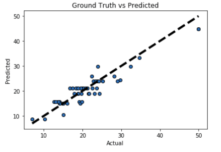
Conclusion :
We can see that our R2 score and MSE are both very good. This means that we have found a best fitting model to predict the median price value of a house. There can be further improvement to the metric by doing some preprocessing before fitting the data. However the task for the post was to provide you sufficient knowledge to implement your first model. You can build over the existing pipeline and report your accuracies.