
Simple Progression Towards Simple Linear Regression
Introduction :
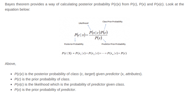
It is a classification technique based on Bayes’ Theorem with an assumption of independence among predictors. In simple terms, a Naive Bayes classifier assumes that the presence of a particular feature in a class is unrelated to the presence of any other feature. For example, a dress may be considered to be a shirt if it is red, printed, and has full sleeve . Even if these features depend on each other or upon the existence of the other features, all of these properties independently contribute to the probability that this cloth is a shirt and that is why it is known as ‘Naive’.
Classification Machine Learning is a technique of learning where a particular instance is mapped against one of the many labels. The labels are prespecified to train your model . The machine learns the pattern from the data in such a way that the learned representation successfully maps the original dimension to the suggested label/class without any more intervention from a human expert.
Naive Bayes model is easy to build and particularly useful for very large data sets. Along with simplicity, Naive Bayes is known to outperform even highly sophisticated classification methods.
4 Applications of Naive Bayes Algorithms
Real time Prediction: Naive Bayes is superfast. Thus, it could be used for making predictions in real time.
Multi class Prediction: This algorithm can predict posterior probability of multiple classes of target variable.
Text classification/ Spam Filtering/ Sentiment Analysis: Naive Bayes classifiers mostly used in text classification (due to better result in multi class problems and independence rule) have higher success rate as compared to other algorithms. As a result, it is widely used in Spam filtering (identify spam e-mail) and Sentiment Analysis (in social media analysis, to identify positive and negative customer sentiments)
Recommendation System: Naive Bayes Classifier along with algorithms like Collaborative Filtering makes a Recommendation System that uses machine learning and data mining techniques to filter unseen information and predict whether a user would like a given resource or not.
Mathematical Explanation :
Problem Statement :
To build a simple generative classification model called Naive Bayes , for predicting the quality of the car given few of other car attributes.
Data details
==========================================
1. Title: Car Evaluation Database==========================================
The dataset is available at “http://archive.ics.uci.edu/ml/datasets/Car+Evaluation”
2. Sources:
(a) Creator: Marko Bohanec
(b) Donors: Marko Bohanec (marko.bohanec@ijs.si)
Blaz Zupan (blaz.zupan@ijs.si)
(c) Date: June, 1997
3. Past Usage:
The hierarchical decision model, from which this dataset is derived, was first presented in
M. Bohanec and V. Rajkovic: Knowledge acquisition and explanation for multi-attribute decision making. In 8th Intl Workshop on Expert
Systems and their Applications, Avignon, France. pages 59-78, 1988.
Within machine-learning, this dataset was used for the evaluation of HINT (Hierarchy INduction Tool), which was proved to be able to
completely reconstruct the original hierarchical model. This,together with a comparison with C4.5, is presented in
B. Zupan, M. Bohanec, I. Bratko, J. Demsar: Machine learning by function decomposition. ICML-97, Nashville, TN. 1997 (to appear)
4. Relevant Information Paragraph:
Car Evaluation Database was derived from a simple hierarchical decision model originally developed for the demonstration of DEX
(M. Bohanec, V. Rajkovic: Expert system for decision making. Sistemica 1(1), pp. 145-157, 1990.). The model evaluates
cars according to the following concept structure:
CAR car acceptability
. PRICE overall price
. . buying buying price
. . maint price of the maintenance
. TECH technical characteristics
. . COMFORT comfort
. . . doors number of doors
. . . persons capacity in terms of persons to carry
. . . lug_boot the size of luggage boot
. . safety estimated safety of the car
Input attributes are printed in lowercase. Besides the target concept (CAR), the model includes three intermediate concepts:
PRICE, TECH, COMFORT. Every concept is in the original model related to its lower level descendants by a set of examples (for
these examples sets see http://www-ai.ijs.si/BlazZupan/car.html).
The Car Evaluation Database contains examples with the structural information removed, i.e., directly relates CAR to the six input
attributes: buying, maint, doors, persons, lug_boot, safety.
Because of known underlying concept structure, this database may be particularly useful for testing constructive induction and
structure discovery methods.
5. Number of Instances: 1728
(instances completely cover the attribute space)
6. Number of Attributes: 6
7. Attribute Values:
buying v-high, high, med, low
maint v-high, high, med, low
doors 2, 3, 4, 5-more
persons 2, 4, more
lug_boot small, med, big
safety low, med, high
8. Missing Attribute Values: none
9. Class Distribution (number of instances per class)
class N N[%]
—————————–
unacc 1210 (70.023 %)
acc 384 (22.222 %)
good 69 ( 3.993 %)
v-good 65 ( 3.762 %)
Tools to be used :
Numpy,pandas,scikit-learn
Python Implementation with code :
Import necessary libraries
Import the necessary modules from specific libraries.
import os

import numpy as np

import pandas as pd

import numpy as np, pandas as pd

import matplotlib.pyplot as plt

from sklearn import metrics , model_selection

## Import the Classifier.

from sklearn.naive_bayes import GaussianNB
Load the data set
Use pandas module to read the bike data from the file system. Check few records of the dataset.
data = pd.read_csv('data/car_quality/car.data',names=['buying','maint','doors','persons','lug_boot','safety','class'])
data.head()
buying    maint       doors      persons  lug_boot safety      class

0              vhigh      vhigh      2              2              small       low          unacc

1              vhigh      vhigh      2              2              small       med         unacc

2              vhigh      vhigh      2              2              small       high        unacc

3              vhigh      vhigh      2              2              med         low          unacc

4              vhigh      vhigh      2              2              med         med         unacc
Check few information about the data set
data.info()
<class 'pandas.core.frame.DataFrame'>
RangeIndex: 1728 entries, 0 to 1727
Data columns (total 7 columns):
buying      1728 non-null object
maint       1728 non-null object
doors       1728 non-null object
persons     1728 non-null object
lug_boot    1728 non-null object
safety      1728 non-null object
class       1728 non-null object
dtypes: object(7)
memory usage: 94.6+ KB
The train data set has 1728 rows and 7 columns.
There are no missing values in the dataset
Identify the target variable
data['class'],class_names = pd.factorize(data['class'])
The target variable is marked as class in the dataframe. The values are present in string format. However the algorithm requires the variables to be coded into its equivalent integer codes. We can convert the string categorical values into a integer code using factorize method of the pandas library.
Let’s check the encoded values now.
print(class_names)

print(data['class'].unique())
Index([u'unacc', u'acc', u'vgood', u'good'], dtype='object')
[0 1 2 3]
As we can see the values has been encoded into 4 different numeric labels.
Identify the predictor variables and encode any string variables to equivalent integer codes
data['buying'],_ = pd.factorize(data['buying'])

data['maint'],_ = pd.factorize(data['maint'])

data['doors'],_ = pd.factorize(data['doors'])

data['persons'],_ = pd.factorize(data['persons'])

data['lug_boot'],_ = pd.factorize(data['lug_boot'])

data['safety'],_ = pd.factorize(data['safety'])

data.head()
buying            maint       doors      persons  lug_boot safety      class

0              0              0              0              0              0              0              0

1              0              0              0              0              0              1              0

2              0              0              0              0              0              2              0

3              0              0              0              0              1              0              0

4              0              0              0              0              1              1              0
Check the data types now :
data.info()
<class 'pandas.core.frame.DataFrame'>
RangeIndex: 1728 entries, 0 to 1727
Data columns (total 7 columns):
buying      1728 non-null int64
maint       1728 non-null int64
doors       1728 non-null int64
persons     1728 non-null int64
lug_boot    1728 non-null int64
safety      1728 non-null int64
class       1728 non-null int64
dtypes: int64(7)
memory usage: 94.6 KB
Everything is now converted in integer form.
Select the predictor feature and select the target variable
X = data.iloc[:,:-1]

y = data.iloc[:,-1]
Train test split :
# split data randomly into 70% training and 30% test

X_train, X_test, y_train, y_test = model_selection.train_test_split(X, y, test_size=0.3, random_state=123)
Training / model fitting
model = GaussianNB()

## Fit the model on the training data.

model.fit(X_train, y_train)
Model parameters study :
# use the model to make predictions with the test data

y_pred = model.predict(X_test)

# how did our model perform?

count_misclassified = (y_test != y_pred).sum()

print('Misclassified samples: {}'.format(count_misclassified))

accuracy = metrics.accuracy_score(y_test, y_pred)

print('Accuracy: {:.2f}'.format(accuracy))
Misclassified samples: 150
Accuracy: 0.71
Algo Advantages :
- It is easy and fast to predict class of test data set. It also perform well in multi class prediction
- When assumption of independence holds, a Naive Bayes classifier performs better compare to other models like logistic regression and you need less training data.
- It perform well in case of categorical input variables compared to numerical variable(s). For numerical variable, normal distribution is assumed (bell curve, which is a strong assumption).
Algo Disadvantages :
- If categorical variable has a category (in test data set), which was not observed in training data set, then model will assign a 0 (zero) probability and will be unable to make a prediction. This is often known as “Zero Frequency”. To solve this, we can use the smoothing technique. One of the simplest smoothing techniques is called Laplace estimation.
- On the other side naive Bayes is also known as a bad estimator, so the probability outputs from predict_proba are not to be taken too seriously.
- Another limitation of Naive Bayes is the assumption of independent predictors. In real life, it is almost impossible that we get a set of predictors which are completely independent.
Way ahead :
In this article, we looked at one of the supervised machine learning algorithm “Naive Bayes” mainly used for classification. The model actually has a 71% accuracy score, since this is a very simplistic data set with distinctly separable classes. But there you have it. That’s how to implement Naive-Baiyes with scikit-learn. Load your favorite data set and give it a try!. From here, all you need is practice.
Further, I would suggest you to focus more on data pre-processing and feature selection prior to applying Naive Bayes algorithm.