Speeding Up and Benchmarking Logistic Regression With PCA
Introduction :
When the data becomes too much in its dimension then it becomes a problem for pattern learning. Too much information is bad on two things : compute and execution time and quality of the model fit. When the dimension of the data is too high we need to find a way to reduce it. But that reduction has to be done in such a way that we maintain the original pattern of the data. The algorithm that we are going to discuss in this article does the similar job. The algorithm is quite famous and widely used in varieties of tasks. Its name is Principal Component Analysis aka PCA.
The main purpose of principal component analysis is the analysis of data to identify patterns and finding patterns to reduce the dimensions of the dataset with minimal loss of information.
PCA is used to transform a high-dimensional dataset into a smaller-dimensional subspace ;into a new coordinate system.In the new coordinate system, the first axis corresponds to the first principal component, which is the component that explains the greatest amount of the variance in the data.
In simple words, principal component analysis is a method of extracting important variables known as principal components from a large set of variables available in a data set. It captures as much information as possible from the original high dimensional data. It represents the original data in terms of its principal components in a new dimension space.
Summary of PCA :
Applications of PCA :
- Visualisation
- Denoising
- Data Compression
- Speeding up ML algorithms
Problem Statement :
Speed up Handwriting recognition learning
Solution :
We will solve this problem by forming the a classification pipeline on MNIST dataset.
About the Dataset :
The MNIST database of handwritten digits, available from this page, has a training set of 60,000 examples, and a test set of 10,000 examples. It is a subset of a larger set available from NIST. The digits have been size-normalized and centered in a fixed-size image. It is a good database for people who want to try learning techniques and pattern recognition methods on real-world data while spending minimal efforts on preprocessing and formatting.
Four files are available on this site:
● train-images-idx3-ubyte.gz: training set images (9912422 bytes)
● train-labels-idx1-ubyte.gz: training set labels (28881 bytes)
● t10k-images-idx3-ubyte.gz: test set images (1648877 bytes)
● t10k-labels-idx1-ubyte.gz: test set labels (4542 bytes)
The MNIST database of handwritten digits is available on the following website: MNIST Dataset
Train a model with all components
Import necessary packages :
from sklearn.datasets import fetch_mldata

from sklearn.decomposition import PCA

from sklearn import metrics

from sklearn.model_selection import train_test_split

import pandas as pd

from sklearn.linear_model import LogisticRegression

from sklearn.preprocessing import StandardScaler

import numpy as np
Load the Dataset :
# You can add the parameter data_home to wherever to where you want to download your data

mnist = fetch_mldata('MNIST original')
Check data information:
print(mnist.data.shape)
print(mnist.COL_NAMES)
print(mnist.target.shape)
(70000, 784)
['label', 'data']
(70000,)

[0. 1. 2. 3. 4. 5. 6. 7. 8. 9.]
There are 70,000 records of 784 dimensions. The labels are a 70,000 dimensional vector. The dimension has been exported under name ‘data’ and labels are exported as ‘target’.
Split the data into train/test :
# test_size: what proportion of original data is used for test set
train_img, test_img, train_lbl, test_lbl = train_test_split(
mnist.data, mnist.target, test_size=1/7.0, random_state=0)
Standardize the data :
scaler = StandardScaler()

# Fit on training set only.
scaler.fit(train_img)
# Apply transform to both the training set and the test set.
train_img = scaler.transform(train_img)
test_img = scaler.transform(test_img)
Notice that we have done the fitting on the training set only and then applied that to the test data as well.
Initialize a becnchmarking dataframe :
Let’s initialise a pandas dataframe that would hold :
- Variance : The variance of the original data that is retained
- N_components : number of principal components
- Timing : time to fit training
- Accuracy : Accuracy obtained
We will capture the above attributes from each experiment run .
benchmark_cols = ['Variance retained','n_Components','Time(s)','Accuracy_percentage']
benchmark = pd.DataFrame(columns = benchmark_cols)
Train the model with all data:
Train a logistic regression on all data and record the training time and accuracy.
The variance and num of components will be obviously 1.0 and 784.
variance = 1.0
n_components = train_img.shape[1]
logisticRegr = LogisticRegression(solver = 'lbfgs')
start = time.time()
logisticRegr.fit(train_img, train_lbl)
end =  time.time()
timing = end-start
# Predict for Multiple Observations (images) at Once
predicted = logisticRegr.predict(test_img)
# generate evaluation metrics
accuracy = (metrics.accuracy_score(test_lbl, predicted))
a = dict(zip(benchmark_cols,[variance,n_components,timing,accuracy]))
benchmark = benchmark.append(a,ignore_index=True)

print(benchmark)
Variance retained  n_Components    Time(s)  Accuracy_percentage
0               1.00         784.0  72.379794               0.9155
Training on total was done in ~73 seconds and it yielded an accuracy of 91.%.
Now let’s train on the data with reduced variance.We will use PCA to reduce the no of components.
Decide on the variance percentages :
Fix the variances for which we would conduct the experiments .
variance_list = [0.95,0.90,0.85,0.80,0.75,0.70]
We would check how much time is taken to build a ML model having the specified data variances .
Define a function to run the same model with various variances :
def benchmark_pca(variance,train_img,train_lbl,test_img,test_lbl):
    global benchmark
    print(train_img.shape)
    pca = PCA(variance)
    pca.fit(train_img)
    n_components = pca.n_components_
    train_img = pca.transform(train_img)

    # pca.fit(test_img)
    test_img = pca.transform(test_img)
    logisticRegr = LogisticRegression(solver = 'lbfgs')
    start = time.time()
    logisticRegr.fit(train_img, train_lbl)
    end =  time.time()

    timing = end-start

    # Predict for Multiple Observations (images) at Once
    predicted = logisticRegr.predict(test_img)

    # generate evaluation metrics
    accuracy = (metrics.accuracy_score(test_lbl, predicted))
    #return
    a = dict(zip(benchmark_cols,[variance,n_components,timing,accuracy]))
    benchmark = benchmark.append(a,ignore_index=True)

for variance in variance_list:
    benchmark_pca(variance,train_img,train_lbl,test_img,test_lbl)
Variance retained  n_Components    Time(s)  Accuracy_percentage
0               1.00         784.0  72.379794               0.9155
1               0.95         330.0  39.592324               0.9200
2               0.90         236.0  30.176633               0.9169
3               0.85         184.0  23.074336               0.9154
4               0.80         148.0  19.963392               0.9127
5               0.75         120.0  19.286882               0.9105
6               0.70          98.0  17.231295               0.9075
Let’s plot the relation between accuracy and other elements.
import matplotlib.pyplot as plt
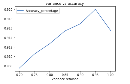
benchmark.plot(x=0,y=-1)
plt.title("variance vs accuracy")
import matplotlib.pyplot as plt
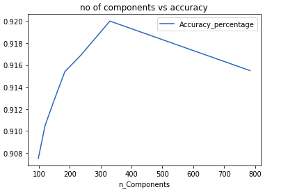
benchmark.plot(x=1,y=-1)
plt.title("no of components vs accuracy")
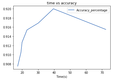
import matplotlib.pyplot as plt
benchmark.plot(x=2,y=-1)
plt.title("time vs accuracy")